
Unlike other methods probabilistic machine learning is based on
one consistent principle which is used throughout the entire
inference procedure. Probabilistic methods approach inference of
latent variables, model coefficients, nuisance parameters and
model order essentially by applying
Bayesian Theory. Hence we may
treat all unknown variables identically which is mathematically nice.
For computational reasons a fully probabilistic model might not be
feasible. In such situations we have to use approximations. Obviously
for a methodology that has to stand the test in an empirical discipline,
a mathematical consistency argument is not too convincing. So why should
one use probabilistic methods?
Advantages of probabilistic models
- Fully probabilistic models avoid "black box" characteristics.
We may instantiate arbitrary sets of variables and for
diagnosis purposes infer the distributions over (or expectations of)
other variables of interest and thus obtain some insight how we obtain a
particular decision.
- Using a probabilistic model is relatively easy.
Inference (if properly implemented) should be insensitive to the
setting of all "fiddle parameters" and will thus provide results
that are close to optimal. An example that relies on this property is
adaptive inference which I have used for our
adaptive classification.
- Probabilistic models provide means for intelligent
sensor fusion
which allows e.g. to combine information that is known with
different certainty.
Disadvantages of probabilistic models
- Inference of fully probabilistic models can be slow.
- Inferring probabilistic models inevitably requires to model
distributions. Sometimes this can be more than we are asked for.
The basic idea of Bayesian sensor fusion is to take uncertainty of
information into account. In machine learning the seminal papers were
those by (MacKay 1992) who discussed the
effects of model uncertainty. In (Wright 1999)
these ideas were later extended to input uncertainty. Related ideas
have been used by
(Dellaportas & Stephens 1995), who
discuss models for errors in observables. I got interested in these
issues in the context of hierarchical models where model parameters
of a feature extraction stage are used for diagnosis or
segmentation purposes. Such models are e.g. used for sleep analysis
or also in the context of BCI. In a Bayesian sense these features
are latent variables and should be treated as such. Again this is
a consistency argument which has to be examined for its practical
relevance.
 In order to obtain a hierarchical model that does sensor fusion we
simply regard the feature extraction stage as latent space and
integrate (marginalize) over all uncertainties.
The left figure compares a sensor fusing DAG with current practice in many
applications of probabilistic modeling that regard extracted
features as observations. I reported on a first attempt to approach
this problem in (Sykacek 1999)
which is in more detail described in section 4 in my
Ph.D. thesis.
In order to obtain a hierarchical model that does sensor fusion we
simply regard the feature extraction stage as latent space and
integrate (marginalize) over all uncertainties.
The left figure compares a sensor fusing DAG with current practice in many
applications of probabilistic modeling that regard extracted
features as observations. I reported on a first attempt to approach
this problem in (Sykacek 1999)
which is in more detail described in section 4 in my
Ph.D. thesis.
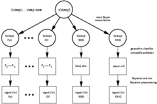
In order to see that a latent feature space has practical advantages, we
consider a very simple case where two sensors are fused in a naive Bayes
manner to predict the posterior probability in a two class problem.
 The model is similar to the one in the graph used above, however with two
latent feature stages that are, conditional on the state of interest t,
assumed to be independent. The plot on the right illustrates the effect
of knowing one of the latent features with varying precision.
Conditioning on a best estimate results obviously in
probabilities that are independent of the precision. We hence obtain a
flat line with a probability of class "2" of about 0.27.
Marginalization changes this probability. Depending on how much the uncertainties
differ, we can, as is illustrated in this figure, also obtain different
predicted states. We may thus expect to improve in such cases where the
precision of the distributions in the latent feature
space varies. We have successfully applied a HMM based latent feature space model
to classification of segments of multi sensor time series. Such problems arise in
clinical diagnosis (sleep classification) and in the context of brain computer
interfaces (BCI). A MCMC implementation and evaluation on synthetic and BCI data
has been published in (Sykacek & Roberts 2002 a).
This work was also the topic of a talk I gave at the
NCRG in Aston in July 2002. A pdf version of the slides being available
here. Recently
(Beal et al. 2002) have applied similar
ideas to sensor fusion of audio and video data.
The model is similar to the one in the graph used above, however with two
latent feature stages that are, conditional on the state of interest t,
assumed to be independent. The plot on the right illustrates the effect
of knowing one of the latent features with varying precision.
Conditioning on a best estimate results obviously in
probabilities that are independent of the precision. We hence obtain a
flat line with a probability of class "2" of about 0.27.
Marginalization changes this probability. Depending on how much the uncertainties
differ, we can, as is illustrated in this figure, also obtain different
predicted states. We may thus expect to improve in such cases where the
precision of the distributions in the latent feature
space varies. We have successfully applied a HMM based latent feature space model
to classification of segments of multi sensor time series. Such problems arise in
clinical diagnosis (sleep classification) and in the context of brain computer
interfaces (BCI). A MCMC implementation and evaluation on synthetic and BCI data
has been published in (Sykacek & Roberts 2002 a).
This work was also the topic of a talk I gave at the
NCRG in Aston in July 2002. A pdf version of the slides being available
here. Recently
(Beal et al. 2002) have applied similar
ideas to sensor fusion of audio and video data.
The image on the right shows a
directed acyclic graph of
our BCI classifier. Every time instance n represents a
second of EEG and the corresponding cognitive state. At instance n,
we are given a
distribution over the parameter vector w
n-1
a new observation y
n. Assuming a two state BCI (e.g. we want to
discriminate between cortical activity in the left and right motor cortex),
y
n ∈ [0,1] and the BCI classifier predicts the probability
P(y
n|D). We use D to denote all
past observations
including previous sessions. Data D results in a Gaussian distribution
over the previous parameter p(w
n-1|D) which has mean
û
n-1 and precision matrix Λ
n-1. As soon as we
observe y
n we can update the distribution to obtain
p(w
n-1|D, y
n). The hyper parameter λ can be
regarded as a
forgetting factor that controls the amount of
tracking of the algorithm. Rather than setting its value directly, we use
a hierarchical setup. We specify a Gamma prior p(λ|α, β)
and infer the posterior distribution
p(λ|y
n-N,...y
n-1,α, β).
This assumes a stationary
adaptation rate λ within a
window of size N.
The adaptive classifier
requires to specify values for α, β and the window length N. Based on
investigations with stationary data and with data with
known
non-stationary behavior we suggest to use α=0.01, β=10
-4 and N=10.
Results on a synthetic data set with these and similar settings are shown in the
figure on the left. The above plot illustrates the expectation of λ
under the posterior. The second plot shows the instantaneous generalization
accuracy. The data set is stationary - apart from a non-stationary behavior
at sample 500, where we
flip the labels.
Although different values of N lead to different estimates of the optimal
adaptation rate, the effect on the generalization accuracy is small and the
best compromise between rapid tracking and high stationary accuracy is obtained
with a window of size 10. As a final comment we would like to mention that
these settings allow that the algorithm is done in real time - a vital property
to be useful for a BCI.
- (Beal et al. 2002)
-
M. J. Beal, H. Attias and N. Jojic.
A Self-Calibrating Algorithm for Speaker Tracking Based on
Audio-Visual Statistical Models.
In Proc. Int. Conf. on Acoustics Speech and Signal Proc.
(ICASSP), May 2002.
- (Bernardo & Smith 1994)
-
J. M. Bernardo and A. F. M. Smith. Bayesian Theory.
John Wiley & Sons, Chichester UK, 1994.
- (Dellaportas & Stephens 1995)
-
P. Dellaportas and S. A. Stephens. Bayesian analysis of errors-in-variables
regression models. Biometrics, 51:1085-1095, 1995.
- (MacKay 1992)
-
D. J. C. MacKay. Bayesian interpolation. in Neural Computation,
pages 415-447, 1992.
- (Sykacek 1999)
-
Learning from uncertain and probably missing data.
Peter Sykacek, OEFAI. An abstract is available on the
workshop homepage.
- (Sykacek et al. 2003 b)
-
P. Sykacek, I. Rezek and S. J. Roberts. Bayes Consistent
Classification of EEG Data by Approximate Marginalisation.
In S. J. Roberts and R. Dybowski editors. Applications of
Probabilistic Models for Medical Informatics and Bioinformatics,
pages to appear, Springer Verlag, 2003.
- (Sykacek & Roberts 2003)
-
P. Sykacek and S. J. Roberts.
Adaptive classification by variational Kalman filtering.
In S.Thrun, S. Becker and K. Obermayer, editors, Advances
in Neural Information Processing Systems 15, pp 737-744,
MIT press, 2003.
- (Sykacek & Roberts 2002)
-
P. Sykacek and S. Roberts. Bayesian time series classification. In
T.G. Dietterich, S. Becker, and Z. Ghahramani, editors, Advances in
Neural Processing Systems 14, pages 937–944. MIT Press, 2002.
- (Wright 1999)
-
W. A. Wright. Bayesian approach to Neural-Network modeling with input uncertainty.
IEEE Trans. Neural Networks, 10:1261-1270, 1999.
Brain computer interface summarizes all components necessary to
establish a thought based human-computer communication channel.
There are two main directions in BCI research.
A BCI can be based on P300 related events with
(Farwell & Donchin 1988) being one of the first
references. The second class of BCI is based on voluntary
control of cognitive tasks, with
(Birbaumer et al. 1999) ,
(Pfurtscheller et al. 1993) and
(Wolpaw et al. 1991) being the dominating research groups
using this paradigm. Our BCI also follows this second line of
thought. PARG members are involved in BCI research for
about five years
(Roberts et al. 1998). Having joined PARG and Oxford University
in September 2000, I work on BCI since then.
In order to make our BCI simple to use, we record a few EEG channels
only (four at most). Our recording equipment is based on a
Gtec amplifier
and an AD converter from
national instruments.
The low number of EEG channels requires the channel
positions to be appropriately synchronized with the cortical area
activated during the cognitive task under consideration. Thus our
experimental protocol
(Curan et al. 2003) requires input from cognitive psychology which
in our case is provided by Prof. Stokes and her colleagues from the
Research Department of the Royal Hospital for Neuro Disability,
Putney, London.

According to the taxonomy used in
(Wolpaw et al. 2002),
our research concentrates on the
signal processing part
of the BCI. In particular we regard the BCI as a feedback loop
with
two adaptive entities: on one hand the BCI user will
adapt such as to maximize correct feedback; on the other hand machine
learning techniques are inherently adaptive as well.
The inevitable adaptation of the user requires signal processing concepts
that can
track non-stationary events. Thus the working hypothesis
for our BCI 2003 is that it must use
adaptive inference.
Probabilistic methods summarizes all approaches that are
consistent with an axiomatic framework that result in
Bayesian theory. Agreed - consistency is
nice
but from an application point of
view, where
performance is the only relevant measure, not
necessary. However probabilistic methods have several other
properties which make them extremely useful for many problems
we encounter in the signal processing part of a BCI. To mention the
most important:
- Model selection can be done consistently by using
probabilistic methods. The true Bayesian approach
(Sykacek 2000 b) would
even go further and combine all models under consideration
according to their probability under the training data.
In the context of our BCI this has in
(Curan et al. 2003) been applied successfully
to find the optimal complexity of the BCI classifier.
- Probabilistic methods are inherently coupled with the concept of
integrating out uncertainties (this refers to mathematical
integration). In a multi sensor environment
(e.g. multiple EEG channels) integration has the advantage to
result in certainty based sensor fusion. Applied to BCI
data
(Sykacek & Roberts 2002 a)
this leads to a significant improvement in bit rate. More
detailed information on that issue is available on my
machine learning research page in section
Bayesian sensor fusion.
- A problem with non probabilistic BCI systems is that model fitting requires
tuning of several parameters like penalty constants or model orders.
Setting these parameters requires validation data and many time consuming
repetitions of the model fitting process. The performance of the trained model
depends critically on these parameters and requires expert knowledge.
In a probabilistic world such parameters are called hyper parameters.
The probabilistic framework provides means for inferring these hyper
parameters together with model parameters in one go. Although we still
have to choose some parameters, a well designed hierarchical setup makes inference
less sensitive to their values. This aspect of probabilistic methods is of vital
importance for our BCI research.
In order to assess the effects on the bit rates of BCI's, we compare in
(Curan et al. 2003)
the communication bandwidth we may achieve with different cognitive tasks
(Curran & Stokes 2003).
We base comparisons on generalization accuracies obtained for independent test data.
Differences are assessed for statistical significance using McNemar's test, a
test for analyzing paired results that can be found in (Ripley 1996).
In order to allow comparisons with other BCI systems, we also report bit rates as
is suggested in (Wolpaw et al. 2000). The BCI
experiments in this study were done by 10 young, healthy
and untrained subjects. They are based on 3 cognitive tasks:
an auditory imagination, an imagined spatial navigation task and an
imagined right motor task. Each experiment consists of 10
repetitions of alternating pairs of these tasks each of which have been done for seven
seconds. EEG recordings are obtained from two electrode sites: T4, P4 (right
tempero-parietal for spatial and auditory tasks), C3' , C3" (left motor area for right
motor imagination). The ground electrode is placed just lateral to the left mastoid process.
| comparison | accuracy (a) | bit/s (a) | accuracy (b) |
bit/s (b) | Pnull |
| (a) vs. (b) | 74 % | 0.173 | 69 % | 0.107 |
<<0.01 |
| (a) vs. (c) | 74 % | 0.173 | 71 % | 0.131 |
<0.01 |
| (a) vs. (d) | 74 % | 0.173 | 71 % | 0.131 |
0.01 |
| (b) vs. (c) | 69 % | 0.107 | 71 % | 0.131 |
0.02 |
| (b) vs. (d) | 69 % | 0.107 | 71 % | 0.131 |
0.03 |
| (c) vs. (d) | 71 % | 0.131 | 71 % | 0.131 |
0.40 |
An investigation of different classification paradigms reveals that on this data the BCI
classifiers perform significantly better, when allowing for a nonlinear decision boundary.
The method applied in this comparison uses autoregressive features (AR) extracted from successive
segments of EEG. We use a generative classifier that predicts probabilities of cognitive states.
Table Comparison of different tasks summarizes the results of
this comparison. Task pairing (a) refers to the combination navigation - auditory, task
pairing (b) refers to the combination navigation - right motor, task pairing (c) refers to the
combination auditory - right motor and task pairing (d) refers to the combination left motor -
right motor, which we include in order to allow for a comparison with these classical tasks.
Our results allow to conclude that (a) vs. (b) result in slightly better correct classification
rates as the classical imagined motor task. However, since we can extract information about
the cognitive state in all cases, the main conclusion is that we might significantly increase
the bit rate of BCI systems by using more than two cognitive tasks. For more details on this
study we refer to (Curan et al. 2003).
Bayesian sensor fusion for offline BCI
Probabilistic models can be used to describe many architectures that have been applied to static
and adaptive BCI systems. Examples are Hidden Markov models, that have been successfully
applied to BCI in (Obermeier et al. 2001). Probabilistic
models have also been quite popular tools in the
machine learning and statistics community. Recently these communities have investigated
efficient algorithms that allow inference of very complex models. These findings are of
interest for the BCI community since they allow us to go beyond classical time series models
and by that improve different aspects of BCI systems. We have recently evaluated two such
generalizations in the context of BCI systems. Coupled HMM's are generalizations of ordinary
HMM's, where two hidden state sequences are probabilistically coupled using arbitrary
lags. In (Rezek et al. 2002) these models have
been applied to movement planning and shown to outperform classical HMM's.
Another modification of HMM's was proposed in
(Sykacek & Roberts 2002), where we follow
probabilistic principles and suggest that classifications based on feature extraction
(like the use of spectral
representations or AR models as used in our BCI) have to regard the features as latent
variables. Hence inference and predictions need to marginalize over this latent space.
The practical advantage of the proposed architecture is that both the feature and the model
uncertainty (the latter means the uncertainty about model order) are automatically taken
into consideration. This effects model estimation and prediction and results in automatic
artefact moderation and thus in intelligent sensor fusion. The idea exploits a property
found by marginalization (i.e. integration over the distribution) over (at least two)
uncertain latent variables estimated from two sensor signals (e.g. EEG recorded at different
electrode sites). Depending on the variance of the distribution, we will obtain different
posterior probabilities.
Section Bayesian sensor fusion
illustrates the effect using two sensor signals Xa and Xb and the
state of interest (e.g. the cognitive state we want to predict) y. We see how the posterior
probability depends on the variance. The effect may even result in a different assessment
w.r.t. the predicted state.
The application of such a marginalization idea to BCI is illustrated in table
BCI with fully Bayesian method. We
illustrate results obtained with this paradigm using two task pairings of the study
reported in our neuro-cognitive study. We compare the
generalization accuracies of the fully probabilistic model (full Bayes) with those
of a classical approach that does feature extraction separately.
Table BCI with fully Bayesian method shows also
the probabilities of the null hypothesis Pnull that the results are equal
(McNemar's test).
We may thus conclude that a fully Bayesian approach significantly outperforms
classifications obtained when conditioning on feature estimates. Despite having
found that a fully Bayesian approach improves BCI performance,
the proposed method has the disadvantage of not being directly applicable to online BCI.
The computational complexity simply does not allow that. Hence we investigated an
approximation which can be used in real time and nevertheless achieve the desired
effects (Sykacek et al. 2003 b) .
| classical model | full Bayes | |
| task pair | Accuracy | bit rate b/s | Accuracy |
bit rate b/s | Pnull |
| (d) | 75.9% | 0.20 | 81.4% | 0.31 | 0.04 |
| (a) | 76.2% | 0.21 | 84.5% | 0.38 |
<<0.01 |
Current BCI architectures developed by other research groups rely on assuming that
the EEG generated during cognitive tasks shows stationary behavior.
This assumption must be wrong for several reasons:
-
There are technical problems with the electrolyte fluids used for electrode placement.
It simply dries out and thus changes impedance. Hence both signal amplitudes and dynamics
are subject to temporal variations during a BCI session.
-
Both learning (habitation) effects and fatigue (Note at this point that sleep staging is
entirely based on variations of EEG dynamics.) change the dynamics during and between BCI
sessions.
We thus suggest a fully adaptive approach for the translation algorithm that, even in short
time use of a BCI, resulted in higher communication bandwidth than conventional
static BCI's.
Probabilistic models can be of advantage in describing algorithms for adaptive
BCI systems. A graph structure that illustrates such an approach is shown in my section on
adaptive classification.
We assume a model that predicts the probabilities of cognitive states and regard
the parameters of the classifier are regarded as latent variables in a first order
Markov process. The solution in a linear Gaussian case are the well known Kalman
filter equations. In our case the non-linearity introduced by predicting probabilities
requires us to use an approximation. We suggest for that purpose a variational
technique and thus obtain variational Kalman filtering as an inference method
(Sykacek & Roberts 2003) .
Variational methods (Jordan et al. 1999,
Attias 1999) are attractive for BCI systems because
compared with Laplace approximations (as e.g. used for classification problems in
(Penny & Roberts 1999),
they allow for more flexibility and contrary to particle filters they still provide a
parametric form of the posterior. Having a parametric posterior is important since it
allows efficient real time implementations. We apply this algorithm to
features extracted from EEG. My favorite approach is to use a lattice filter
representation of auto regressive parameters since they have in
(Sykacek et al. 1999 c)
been found superior to other feature extraction techniques including conventional AR
parameters. Results applying the variational Kalman filter classifier to the BCI data
described in our neuro-cognitive study,
are summarized in table Adaptive BCI. The last column
are the probabilities of the null hypothesis Pnull that the results are equal
(McNemar's test).The results suggest that a truly adaptive BCI (column vkf) significantly
outperforms the equivalent static method (column vsi). A detailed description of our
adaptive translation algorithm and a thorough evaluation can be found in
(Sykacek et al. 2003 c).
| Generalization results |
| vkf | vsi | |
| Cognitive task | Accuracy | bit/s | Accuracy | bit/s |
Pnull |
| navigation/auditory | 86% | 0.42 | 83% | 0.34 |
0.02 |
| navigation/movement | 80% | 0.28 | 80% | 0.28 |
0.31 |
| auditory/movement | 78% | 0.24 | 76% | 0.21 |
<<0.01 |
- (Curran et al. 2003)
-
E. Curran, P. Sykacek, M. Stokes, S. J. Roberts, W. Penny,
I. Johnsrude and A. M. Owen. Cognitive tasks for driving a Brain
Compute Interfacing System. In IEEE Trans. Neural Systems and
Rehabilitation Engineering, pages to appear, 2003.
- (Sykacek 2003 b)
-
P. Sykacek. Brain Computer Interfacing: State of the Art, Probabilistic Advances and
Future Perspectives. Technical Report, available in
pdf and as
gzipped postscript.
- (Sykacek 2003 a)
-
P. Sykacek. Towards Adaptive BCI. Presentation
at the NCAF meeting on human computer interaction,
3-4 September 2003, Cambridge, UK.
- (Sykacek et al. 2003 c)
-
P. Sykacek, S. J. Roberts and M. Stokes. Adaptive BCI based
on variational Bayesian Kalman filtering: an empirical evaluation.
In IEEE Trans. Biomedical Engineering, pages to appear, 2003.
A poster describing the
adaptive BCI was awarded in the "best engineering" category at the BCI
workshop 2002 in Albany, NY, June 12-17.
- (Sykacek et al. 2003 b)
-
P. Sykacek, I. Rezek and S. J. Roberts. Bayes Consistent
Classification of EEG Data by Approximate Marginalisation.
In S. J. Roberts and R. Dybowski editors. Applications of
Probabilistic Models for Medical Informatics and Bioinformatics,
pages to appear, Springer Verlag, 2003.
- (Sykacek et al. 2003 a)
-
P. Sykacek, S. J. Roberts, M. Stokes, E. Curran, M. Gibbs
and L. Pickup. Probabilistic methods in BCI research.
In IEEE Trans. Neural Systems and Rehabilitation Engineering,
pp. 192--195, 2003.
References
- (Attias 1999)
-
H. Attias. Inferring parameters and structure of latent variable
models by variational Bayes. in Proceedings of
the Fifteenth Annual Conference on Uncertainty in Artificial
Intelligence (UAI--99),
pages 21-30, 1999.
- (Birbaumer et al. 1999)
-
N. Birbaumer, N. Ghanayim, T. Hinterberger, I. Iversen,
B. Kotchoubey, A. Kübler, J. Perelmouter, E. Taub and H. Flor.
A spelling device for the paralysed. Nature ,
398:297-298, 1999.
- (Curran & Stokes 2003)
-
E. Curran and M. Stokes. Learning to control brain activity:
A review of the production and control of EEG components for driving
brain-computer interface (BCI) systems. Brain and Cognition,
51: 326–335, 2003.
- (Farwell & Donchin 1988)
-
L. A. Farwell and E. Donchin. Talking off the top of your head:
Toward a mental prosthesis utilizing event-related brain
potentials. Electroencephalography and Clinical
Neurophysiology , 70:510-523, 1988.
- (Jordan et al. 1999)
-
M. I. Jordan, Z. Ghahramani, T. S. Jaakkola, and L. K.
Saul. An introduction to variational methods for graphical models. In
M. I. Jordan, editor, Learning in Graphical Models. MIT Press,
Cambridge, MA, 1999.
- (Obermeier et al. 2001)
-
B. Obermeier, C. Guger, C. Neuper, and G. Pfurtscheller.
Hidden Markov models for online classification of single trial EEG. Pattern
Recognition Letters, pages 1299–1309, 2001.
- (Penny & Roberts 1999)
-
W. Penny and S. J. Roberts. Non stationary logistic regression. In Proceedings
of the IJCNN 1999, 1999.
- (Pfurtscheller et al. 1993)
-
G. Pfurtscheller, D. Flotzinger and J. Kalcher. Brain-Computer
Interface - a new communication device for handicapped people.
Journal of Microcomputer Applications , pages 293-299,
1993.
- (Rezek et al. 2002)
-
I. Rezek, M. Gibbs, and S. Roberts. Maximum a posteriori
estimation of coupled hidden Markov models. Advances in Neural Networks for
Signal Processing, page to appear, 2002.
- (Ripley 1996)
- B. D. Ripley. Pattern Recognition and Neural Networks. Cambridge
University Press, Cambridge, 1996.
-
- (Roberts et al. 1998)
-
S. J. Roberts, W. Penny and I. Rezek. Temporal and Spatial
Complexity Measures for EEG-based Brain-Computer Interfacing.
Medical & Biological Engineering & Computing , 37(1),
pages 93-99, 1998.
- (Wolpaw et al. 1991)
-
J. R. Wolpaw, D. J. McFarland, D. J. Neat and C. A. Froneis.
An EEG-based Brain-Computer Interface for Cursor Control.
Electroencephalography and Clinical Neurophysiology ,
78:252-259, 1991.
- (Wolpaw et al. 2002)
-
J. R. Wolpaw, N. Birbaumer, D. J. McFarland, G. Pfurtscheller and T. M. Vaughan.
Brain-computer interfaces for communication and control.
Clinical Neurophysiology, 113:767-791, 2002.
- (Wolpaw et al. 2000)
-
J. R. Wolpaw, N. Birbaumer, W. J. Heetderks, D. J.
McFarland, P. H. Peckham, G. Schalk, E. Donchin, L. A.
Quatrano, C. J. Robinson, and T. M. Vaughan. Brain-Computer Interface
technology: a review of the first international meeting.
IEEE Trans. Rehab. Eng., pages 164–173,2000.
 This page is a summary of my SIESTA activities.
I have looked at various aspects of the EEG model that should lead to the
"core" sleep analyzer. These activities include deriving a Bayesian method
for preprocessing, an investigation of resampling issues, Feature subset
selection and an EEG model based on variational Bayesian techniques that
forms the core of the SIESTA sleep analyzer. We decided for the Bayesian paradigm, since
we found it extremely useful for automatic sleep classification according to Rechtschaffen & Kales rules
(Sykacek et al. 1998 and
Sykacek et al. 2002 a).
I also came up with ideas how to combine models that were built separately for different biosignals.
Below, we will use some acronyms: EEG - electroencephalogram (A signal
obtained by recording from different positions on the scalp. It represents local brain activity.)
EOG - electrooculogram (A signal recorded from the forehead that shows eye movements.)
EMG - electromyogram (A signal recorded from various positions on the human body which represents
the local muscle activity).
This page is a summary of my SIESTA activities.
I have looked at various aspects of the EEG model that should lead to the
"core" sleep analyzer. These activities include deriving a Bayesian method
for preprocessing, an investigation of resampling issues, Feature subset
selection and an EEG model based on variational Bayesian techniques that
forms the core of the SIESTA sleep analyzer. We decided for the Bayesian paradigm, since
we found it extremely useful for automatic sleep classification according to Rechtschaffen & Kales rules
(Sykacek et al. 1998 and
Sykacek et al. 2002 a).
I also came up with ideas how to combine models that were built separately for different biosignals.
Below, we will use some acronyms: EEG - electroencephalogram (A signal
obtained by recording from different positions on the scalp. It represents local brain activity.)
EOG - electrooculogram (A signal recorded from the forehead that shows eye movements.)
EMG - electromyogram (A signal recorded from various positions on the human body which represents
the local muscle activity).
Bayesian preprocessing
The SIESTA analyzer processes EEG with a Bayesian implementation of an AR
lattice filter structure. (Bayesian reflection
coefficients). The difficulty with this representation is the calculation of the
marginal likelihood of the model (i.e. integration of the distribution w.r.t. model
parameters). Preprocessing results in
a-posterior distributions of coefficients and posterior probabilities
for models. Details have first been published in one of our EMBEC abstracts:
(Sykacek et al. 1999 b)
Based on this lattice filter model, I have also tried to obtain a REM/non
REM feature from EMG. However this attempt failed - probably due to the
same reasons why an amplitude based feature could not be derived.
Feature subset selection (FSS)
Since we wanted to make sure that the SIESTA analyzer is built around reasonable
features, we decided to use feature subset selection techniques.
Conventional feature subset selection
FSS is the task of finding a sufficiently large best subset of features
that should capture all details contained in some data relevant to a particular
problem. This definition of FSS forces us to think about several issues:
-
What describes the relevant problem?
-
What is a proper measure of a "best" subset?
-
How do we determine whether a subset is sufficiently large?
We decided that the first question is best answered by considering how
well subsets separate the corner stones of sleep (these are unambiguously
classified segments of wake, deep sleep and REM sleep).
From a technical point of view there are several possibilities for measuring
the quality of feature subsets. We decided to look at the likelihood function
of various classifiers and a nonparametric estimate of an impurity measure
(We measure the Gini index by a k nearest neighbors approach).
Search for the "best" subset was based on suboptimal algorithms (forward selection and
sequential elimination). This was necessary since
the number of features (more than 200) rendered exhaustive search impossible.
The optimal subset size was determined with a statistical significance test. We used
McNemar's test of comparing two paired classifiers and an appropriate p-value. In the
forward selection scheme we add the most promising feature if it increases the
classification accuracy with statistical significance. In the backward elimination
strategy, we remove the least important feature if it does not result in a statistically
significant difference.
Classical FSS Results
As only 5 complete recordings were available until deadline for FSS, we
could not use more than 4 recordings. (I saved one for validation purposes).
A major problem in FSS was that the labels are given for 30 seconds segments
and features are calculated on a one seconds basis. Different features
were calculated on different explicitly or implicitly defined window lengths.
As longer windows will smooth features, the 30 seconds labels will prefer
such features that were calculated using longer windows. As reported in
Den Haag, I could show this effect empirically. Consulting with S. Roberts,
we came to the conclusion that it were best to use only the median sample
of each 30 seconds segment. This should help reducing the effect of different
window lengths.
The results in the following tables are from
(Sykacek et al. 1999 c) .
Subset 1: Gini index and sequential forward selection
| stochastic complexity at C3 |
| Hjorth coefficient at Fp2: cmpl. /(act. * mob) |
Subset 2: Likelihood of logistic regression
| ref. coefficient at C4: 1st. coefficient |
| power spectral density at Fp1: Beta (12.5 Hz - 30.0 Hz) |
| Kalman AR coefficient at C3: 2nd. coefficient |
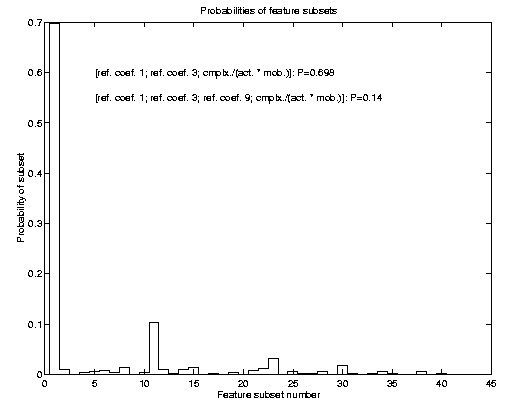
A Bayesian wrapper
 Conventional FSS has a major problem: If two or more (similar sized) subsets
explain the problem equally well, using just one of them is in a Bayesian
sense not consistent with the information provided. The correct approach
would be to integrate out feature subset uncertainty. Consequently we also
applied such a Bayesian technique to the problem of determining relevant
feature subsets. The result of such FSS is a posterior probability
over feature subsets. Prediction would then consider all subsets according
to their posterior probability, which for the SIESTA data is shown in the
image to the left. For further details of this method, I want to refer to
my NIPS 99 preprint (Sykacek 2000 b).
Conventional FSS has a major problem: If two or more (similar sized) subsets
explain the problem equally well, using just one of them is in a Bayesian
sense not consistent with the information provided. The correct approach
would be to integrate out feature subset uncertainty. Consequently we also
applied such a Bayesian technique to the problem of determining relevant
feature subsets. The result of such FSS is a posterior probability
over feature subsets. Prediction would then consider all subsets according
to their posterior probability, which for the SIESTA data is shown in the
image to the left. For further details of this method, I want to refer to
my NIPS 99 preprint (Sykacek 2000 b).
Results Bayesian Wrapper
Subset 3: Bayesian wrapper for C3 only. The posterior probability
of this subset is 0.69
| ref. coefficient at C3: 1st. coefficient |
| ref. coefficient at C3: 3rd. coefficient |
| Hjorth coefficient at C3: cmpl. /(act. * mob) |
The SIESTA sleep analyzer
 The following considerations lead to the chosen architecture for the Siesta analyzer.
- Sleep should be modeled as a three state process (wake, REM and deep sleep). To capture
uncertainty we model probabilities.
- Expert labels might disagree. In this case the independent variables should be used
without label. This required a generative classifier and to model the joint density
over the features extracted from EEG and the "sleep" state.
- We needed an inference scheme that allows for model selection (or model
averaging) without being too difficult to compute on large data sets.
- Later extensions to include models from other sensors (e.g. an EMG model) should be
relatively easy.
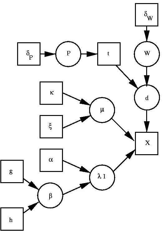
A generative model for classification
 We decided for a model that allows class conditional densities to be mixture
of Gaussians. Together with prior probabilities for class, we thus have a generative model for
EEG features that - via Bayes theorem - allows predicting probabilities for wake, REM and
deep sleep. The corresponding graphical model is illustrated to the left. The basic
architecture was previously used in a maximum likelihood setting e.g.
(Trĺvén 1991). The architecture is a latent variable model consisting of
the "features" x, the class label t and the kernel indicator d. In addition the Bayesian
approach requires us to include all model parameters and hyper parameters as well. These are the
prior probabilities of each class P and the parameters of the mixture model. For the latter
we have W as (class conditional) kernel allocation probabilities, μ as kernel mean and
λ as kernel precision (inverse kernel variance). The remaining variables specify a,
partially hierarchical, prior which is largely influenced by
(Richardson & Green 1997) .
We have δP and δW as prior counts (we use 1) in the Dirichlet
distributions over the corresponding variables P and W. Variables κ and ξ specify a
Gaussian prior over the mean, μ. Variables α and β specify a Gamma prior over the
kernel precisions, λ, where β is itself given a Gamma prior. This hierarchical setting
is suggested by (Richardson & Green 1997) , to make inference
less sensitive to the hyper parameter settings.
We decided for a model that allows class conditional densities to be mixture
of Gaussians. Together with prior probabilities for class, we thus have a generative model for
EEG features that - via Bayes theorem - allows predicting probabilities for wake, REM and
deep sleep. The corresponding graphical model is illustrated to the left. The basic
architecture was previously used in a maximum likelihood setting e.g.
(Trĺvén 1991). The architecture is a latent variable model consisting of
the "features" x, the class label t and the kernel indicator d. In addition the Bayesian
approach requires us to include all model parameters and hyper parameters as well. These are the
prior probabilities of each class P and the parameters of the mixture model. For the latter
we have W as (class conditional) kernel allocation probabilities, μ as kernel mean and
λ as kernel precision (inverse kernel variance). The remaining variables specify a,
partially hierarchical, prior which is largely influenced by
(Richardson & Green 1997) .
We have δP and δW as prior counts (we use 1) in the Dirichlet
distributions over the corresponding variables P and W. Variables κ and ξ specify a
Gaussian prior over the mean, μ. Variables α and β specify a Gamma prior over the
kernel precisions, λ, where β is itself given a Gamma prior. This hierarchical setting
is suggested by (Richardson & Green 1997) , to make inference
less sensitive to the hyper parameter settings.
A Variational generative classifier
For reasons of computational efficiency we decided for a variational implementation for
the generative classifier. The idea follows from implementations by
(Attias 1999) who derives a variational solution for a Gaussian
mixture model or (Gharamani & Beal 2000) who derives a
variational implementation for a mixture of factor analyzers. Variational methods
and the EM algorithm (Dempster et al. 1977) share the same ideas.
The EM algorithm is a special case of a variational lower bound that becomes exact
in the maximum. Unlike the EM, general variational algorithms remain a lower bound.
 To obtain a lower bound, we apply Jensen's inequality, to the log marginal
likelihood. In the simplest case we use a mean field assumption of a factorizing
posterior distribution. Each circular variable in the DAG gets it's own approximate
distribution. Details of how to derive the algorithm can be found in my PhD thesis
(Sykacek 2000 a). As a result of iterating the
variational updates to convergence we obtain a negative free energy for the model
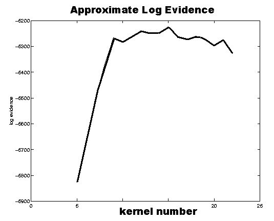
which can be used to guide model selection (Attias 1999).
The plot to the right shows the negative free energies of a generative model for one
of the electrodes (C3) for various numbers of Gaussian kernels. It suggests with very
large probability a model with 15 kernels. More details on the prototype of the
SIESTA sleep analyzer can be found in
(Sykacek et al. 2001).
To obtain a lower bound, we apply Jensen's inequality, to the log marginal
likelihood. In the simplest case we use a mean field assumption of a factorizing
posterior distribution. Each circular variable in the DAG gets it's own approximate
distribution. Details of how to derive the algorithm can be found in my PhD thesis
(Sykacek 2000 a). As a result of iterating the
variational updates to convergence we obtain a negative free energy for the model
which can be used to guide model selection (Attias 1999).
The plot to the right shows the negative free energies of a generative model for one
of the electrodes (C3) for various numbers of Gaussian kernels. It suggests with very
large probability a model with 15 kernels. More details on the prototype of the
SIESTA sleep analyzer can be found in
(Sykacek et al. 2001).
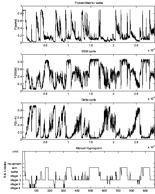
Results
If applied to new data, the SIESTA analyzer calculates probability traces that
characterize the all-night sleep profile. An example plot is illustrated below.
References
- (Attias 1999)
-
H. Attias. Inferring parameters and structure of latent variable
models by variational Bayes. in Proceedings of
the Fifteenth Annual Conference on Uncertainty in Artificial
Intelligence (UAI--99),
pages 21-30, 1999.
- (Dempster et al. 1977)
-
A. P. Dempster, N. M. Laird and D. B. Rubin.
Maximum likelihood from incomplete data via the EM algorithm (with discussion).
In Journal of the Royal Statistical Society B,
pages 1-38, 1977.
- (Dorffner et al. 2000)
-
G. Dorffner, P. Sykacek, S. Roberts, A. Schlögl, A. Värri,
P. Rappelsberger, P. Anderer, G. Klösch, B. Saletu, MJ. Barbanoj,
W. Herrmann, S.-L. Himanen, B. Kemp, T. Penzel, J. Röschke.
Continuous sleep processes and subjective sleep quality - first
results from the SIESTA project. in J. Sleep Res Supplement 1.,
page 55, 2000.
- (Flexer et al. 2002)
-
A. Flexer, G. Dorffner, P. Sykacek, I. Rezek.
An automatic, continuous and probabilistic sleep stager
based on a hidden Markov model.
Applied Artificial Intelligence, 16(3):199-207,2002.
- (Flexer et al. 2000)
-
A. Flexer, P. Sykacek, I. Rezek and G. Dorffner.
Using hidden Markov models to build an automatic,
continuous and probabilistic stager, in S. I. Amari et al.,
Proceedings of the IEEE-INNS-ENNS International Joint
Conference on Neural Networks, IJCNN 2000, Como Italy,
IEEE Computer Society, Vol. III, 627-631, 2000.
- (Ghahramani and Beal 2002)
-
Z. Ghahramani and M. J. Beal. Variational inference for Bayesian mixture
of factor analysers.
Advances in Neural Information Processing Systems 12, 16(3):449-455, 2000.
- (Kemp et al. 1998)
-
Kemp B, Penzel T, Värri A. O., Sykacek P., Roberts S. J.and Nielsen K. D.
EDF: a simple format for graphical analysis results from polygraphic
SIESTA recordings. in J. Sleep Research 7, suppl. 2, page 132, 1998.
- (Richardson and Green 1997)
-
S. Richardson and P. J. Green.
On Bayesian analysis of mixtures with an unknown number of components.
in Journal Royal Stat. Soc. B,
pages 731-792, 1997.
- (Sykacek et al. 2002)
-
P. Sykacek, G. Dorffner, P. Rappelsberger and J. Zeitlhofer.
Improving bio signal processing through modelling uncertainty: Bayes
vs. non-Bayes in sleep staging. Applied Artificial Intelligence,
16(5):395-421,2002.
- (Sykacek et al. 2001)
-
P. Sykacek, S. J. Roberts, I. Rezek, A. Flexer and G. Dorffner.
A probabilistic approach to high resolution sleep analysis.
In G. Dorffner, K. Hornik and H. Bischof, editors,
Proceedings of the International Conference on Neural
Networks (ICANN), pages 617-624, Springer Verlag, 2001.
- (Sykacek 2000 b)
- P. Sykacek. On input selection with reversible jump Markov chain
Monte Carlo sampling. in S. A. Solla and T. K. Leen and K. R. Müller
editors, Advances in Neural Information Processing Systems 12,
pages 638-644, MIT press, 2000.
- (Sykacek 2000 a)
- P. Sykacek. Bayesian inference for reliable biomedical
signal processing, PhD. thesis at the Technical University Vienna,
defended in June 2000.
- (Sykacek et al. 1999 c)
- P. Sykacek, S. J. Roberts, I. Rezek, A. Flexer and G. Dorffner.
Bayesian wrappers versus conventional filters:
Feature subset selection in the Siesta project.
in Proceedings of the European Medical & Biomedical
Engineering Conference, pages 1652-1653, 1999.
- (Sykacek et al. 1999 b)
- P. Sykacek, S. J. Roberts, I. Rezek, A. Flexer and G. Dorffner.
Reliability in preprocessing: Bayes rules Siesta.
in Proceedings of the European Medical & Biomedical
Engineering Conference, pages 1656--1657, 1999.
- (Sykacek et al. 1999 a)
- P. Sykacek, S. J. Roberts, I. Rezek, A. Flexer and G. Dorffner.
Classification in the sampling paradigm: A predictive
approach towards a Siesta sleep analyzer
in Proceedings of the European Medical & Biomedical
Engineering Conference, pages 1660-1661, 1999.
- (Sykacek et al. 1998)
-
P. Sykacek, G. Dorffner, P. Rappelsberger and J. Zeitlhofer.
Experiences with Bayesian learning in a real world application.
in M. I. Jordan and M.J. Kearns and S. Solla editors,
Advances in Neural Information Processing Systems 10,
pages 964-970, 1998.
- (Sykacek et al. 1997)
-
P. Sykacek, G. Dorffner, O. Filz, P. Rappelsberger and J. Zeitlhofer.
Classification of REM sleep periods with artificial neural networks.
in Proc. of Measurement '97, (Smolenice, 1997), pages 327-333,
1997.
- (Trĺvén 1991)
-
H. G. C. Trĺvén. A neural network approach to statistical pattern
classification by ``semiparametric'' estimation of
probability density functions
in IEEE Trans. Neural Networks, pages 366-377, 1991.
This work was done by the authors, while contributing to the
BBSRC funded "Shared Genetic Pathways in Cell Number Control"
research program, which was awarded to the
Department of Pathology,
University of Cambridge, UK.
As the project title suggests, this project investigates
molecular biological processes that control development cycles
in different biological systems. The search for the underlying
genetic markers requires a principled approach that can infer
which genes are of shared importance in several
microarray experiments. We propose for that purpose a fully
Bayesian model for an analysis of shared gene function. The approach assumes
that several microarray experiments with known cross
annotations between transcripts (genes) should be analyzed for
common genetic markers. The implementation described in this
work has in particular the advantage to combine data sets
before applying thresholds and thus the advantage that
the result is independent of that choice. For more information
on the method, we refer to the original paper
(Sykacek et al 2007 a)
and the pdf supplement
(Sykacek et al 2007 b).
Experimental Supplement
Biological Details
The analysis of development processes in many tissues is faced
with several interacting biological processes and a mix of
various cell types. As an example we investigate in this work
the shared biological activity at gene level in a mouse
mammary gland development cycle
(Clarkson et al 2004) and a human endothelial cell
culture with apoptosis induced by serum withdrawal
(Johnson et al 2004). The biological complexity of
the experiments is best visualized, if we mark different
development stages for active biological processes at a macro
level. For the mouse mammary time course, we get the following
table of active processes. During lactation, time is in days
and during involution we use hours.
Biological Processes During Lactation and Involution in Mouse Mammary Development
| Biological Process | L0 | L5 | L10 |
I12 | I24 | I48 | I72 |
I96 |
| Type I Apoptosis | - | - | - | + | + | ? | - |
- |
| Type II Apoptosis | - | - | - | - | - | ? | + |
+ |
| Apoptosis | - | - | - | + | + | + | + |
+ |
| Differentiation | + | + | + | ? | - | - | - |
- |
| Inflammation | ? | - | - | + | + | ? | - |
- |
| Remodeling | -/(?) | - | - | - | - | ? | + |
+ |
| Acute Phase | + | - | - | - | + | + | + |
+ |
We use "+" to indicate that a process is active and "-" to
indicate it's inactivity. A "?" indicates epochs where we are
uncertain about the process activity. A similar though
simpler classification can be obtained for the second
experiment which studies human endothelial cells under serum
deprivation. Duration during serum deprivation is in hours.
Biological Processes in Endothelial Cells Under Serum Withdraw
| Biological Process | control (t0) | t28 |
| Type II Apoptosis | - | + |
| Apoptosis | - | + |
| Differentiation | + | - |
Results
In addition to the results we present in the original paper and in the
pdf supplement, we provide here the top 20 genes we find important to
contribute to both data sets.
Ranking From Shared Analysis of Mammary Development and Endothelial Cells
| Gene Symbol | P(It|D) |
P(G=t|D) | Co-Regulation |
| SAT | 0.99951 | 0.047597 | anti |
| ODC1 | 0.99921 | 0.029237 | co |
| GRN | 0.99921 | 0.029125 | co |
| BSCL2 | 0.99919 | 0.028601 | anti |
| MLF2 | 0.99884 | 0.019988 | anti |
| IFRD2 | 0.99867 | 0.017425 | co |
| BTG2 | 0.99843 | 0.014688 | co |
| CCNG2 | 0.99826 | 0.013274 | co |
| TNK2 | 0.99789 | 0.010943 | anti |
| C9orf10 | 0.99783 | 0.010614 | co |
| HAGH | 0.99764 | 0.0097747 | co |
| PPP2CB | 0.99759 | 0.0095567 | anti |
| SSR1 | 0.99748 | 0.0091528 | co |
| MUT | 0.99747 | 0.0091039 | co |
| DHRS3 | 0.99746 | 0.0090926 | co |
| PSMA1 | 0.99741 | 0.0089018 | anti |
| HBLD2 | 0.99732 | 0.0086073 | co |
| SYPL1 | 0.99724 | 0.0083639 | co |
| C2F | 0.99723 | 0.0083374 | co |
| ATP6V1B2 | 0.99706 | 0.0078419 | anti |
The full gene list in comma separated format is available as
zipped archive. To
check, which biological processes we find attributed to this
list, we follow the suggestion in (Lewin et al. 2006) and use
Fishers exact test to infer significance levels of active gene
ontology (GO) categories from the probabilistic rank list (see
also (Al-Shahrour et
al.)). The resulting GO categories for the gene list of
this shared analysis can be obtained as comb_apo_all.xml in xml
format. This file is compatible with Treemap
- (C) University of Maryland and preserves the parents -
child relationships from the directed acyclic GO graph. Note
that the treeml.dtd file is part of the Treemap package and not
available here. Treemap is under a non commercial license. If it
is unavailable despite that, the xml file can be inspected
with any reasonable web browser.
Software
The software to calculate indicator probabilities that capture
shared gene function comes as collection of MatLab
libraries. The package consists of the main code, which uses the
variational Bayesian approach described in
(Sykacek et al 2007 a)
and additional functions for data handling, output generation
and an EM implementation for regularized probit link
regression used during initialization of all
Q-distributions. To make the software distribution flexible,
all MatLab functions are collected in archives each containing
functions of a particular type. The software is available under
GPL 2 license and comes without any warranty.
Installation
To install the package, one has to download all required
archives, provided as *.zip files or tared gzip archives
(*.tar.gz), unpack the archives and set appropriate MatLab
paths. Scripts using a hypothetical experiment derived from a
mouse testis time course kindly provided by R. Furlong,
demonstrate how to use the library.
Library Files for Shared Analysis (Zip files ending with .zip
instead of .tar.gz are available as well)
|
Library File | Description |
|
helpers.tar.gz | generic helper functions |
|
statsgen.tar.gz | generic statistics functions |
|
mca_base.tar.gz | basic microarray file handling
(loading various microarray data formats) |
|
mca_fuse.tar.gz | generic handling in connection
with shared analysis (cross annotation and output generation) |
|
probitem.tar.gz | Penalized maximum likelihood
(MAP) for probit link regression via an EM algorithm. |
|
combanalysis.glb.hphp.tar.gz |
Variational Bayes for shared analysis of subset probabilities
in probit regression. |
All components required to successfully run the experiment,
will be installed automatically, if one creates a new
directory and then downloads and runs the setup script in that
directory. Linux (Unix) users should use combsyssetup.sh. After
download, you might have to set executable permission by
invoking the command chmod +x combsyssetup.sh. Windows
users should either do the same after installing a cygwin
environment or install the Wget and Unzip packages from
GnuWin32
and then download and run combsyssetup.bat
Note that this will install all required packages and, if run at
later times, install updates.
Tutorial
After having run the script, the installation directory contains
MatLab scripts and data which illustrate the approach discussed in
(Sykacek et al 2007 a).
The data are extracted from a subset of a mouse testis
development time course, kindly provided by R. Furlong. The data
consists of 7 time points: adult day 1 day 5 day 10 day 15 day
23 and day 35, with differential expression measured against the
adult generation.
Data Files for the Tutorial
To illustrate all steps from cross annotation
to generation of gene lists, we divided this data artificially
into two "experiments". One experiment contains the samples of
the adult generation and days 1 and 15. Here we use the original
gene ids. We assume that the biological state change is between
adult and the other two development periods. The corresponding
data file is called "exp1mca.tsv" and is formatted like
FSPMA normalized raw output:
Gene ids are used as column headers and all samples as rows
below. We also have a corresponding effects description as
"exp1eff.tsv", which is used to generate the labels. The second
experiment contains days 35, 23, 5 and 10 and artificially
modified gene ids, to mimic a situation that requires
between species annotation. Here we assume that the biological
states correspond to days 35 and 23 versus days 5 and 10. The
files are "exp2mca.tsv" for the microarray data and
"exp2eff.tsv" for the labels. Note that the assumption is that
each experiment provides information about differences in late
and early stages of testis development. The analysis goal is
thus similar to a problem, where we attempt to combine two
experiments obtained from different platforms or species. This
requires "cross annotation", which is here done according to the
tab delimited file "crossann.tsv". In general, each row in this
file contains a tuple that provides a unique mapping between
all different unique gene ids one finds in a shared analysis. To
complete the list of files, we provide in addition the tab
delimited file "genespec.csv", which provides for the unique
gene ids in the target genome, a mapping to gene symbols and
descriptions.
Matlab Scripts for the Tutorial
Both artificial experiments have to be cross annotated. This
step will align the gene ids in different experiments and
provide two raw data files and a gene id to symbols and
description annotation in MatLab 6 format. Cross annotation is
done by the MatLab script crossann.m found in the installation
folder.
After cross annotation, we have to prepare for the shared
analysis. This requires to specify a tab delimited text file
("shareanalysis.def") which controls this process. The minimal
requirement is to specify in this control file which
(previously cross annotated) data files should be analyzed for
shared gene function. In addition one can specify a different
set of labels. This is useful to analyze the same data for
different biological classifications. We may also provide
independent test data, which will be used to obtain generalization
errors. Analysis is stared with the script combanalysis.m in
the installation folder. The simulation will, depending on the size
of the problem and the mode of analysis, take up to several
hours (this example is though done in less than one minute or
in a few minutes time, if we want fold results). As a result we get
all simulation output in MatLab format. Details of the
calculated results require to look into the code and to
analyze the variables stored in the MatLab output file.
The last step in an analysis of shared function is to generate
a rank table of shared gene function. This is done with the
script crossann2csv.m found in this folder as well. The result
is a rank list of similar structure as the one provided in the
supplement of the original paper.
All intermediate results generated during a shared analysis is
stored in MatLab 6 format (for Octave compatibility). The
final rank table is a comma separated file.
Summary of result files as generated from this simulation.
|
File Name | Description |
|
exp1.mat, exp2.mat | cross annotated and normalized raw data |
|
crossanngenespec.mat | reordered gene specifications
(id, symbol and description) |
|
state.mat, crosslog.mat | internal log files (see code) |
|
sharetestres.mat | inference result about shared gene function.
This file contains all results including probabilities, predictions
and all Q-distributions found from variational Bayesian inference. |
|
share_test_rank.csv | rank table as comma separated file. |
Adapting Shared Analysis to Different Experiments
To run such an analysis on a different experiment, one must
provide data files structured like those listed in the
data files table. The structure of the
microarray data and the default labels is identical to the
output generated by FSPMA,
which can thus be used as preprocessing tool. In addition, one
has to generate a file which allows cross annotation between all
gene sets that appear in any one data set. If there is only one
set of gene ids, cross annotation should be done anyway, to
obtain the data in the format as expected by runsim.m. In this
case all parts in runsim.m that specify the shared analysis will
refer to the same gene id column. Inference of shared gene
function requires in addition a control file similar to
shareanalysis.def. Finally one has to adjust all script files in
the script files summary to meet the
different requirements.
Acknowledgments
This page describes joint work with
R. Clarkson,
C. Print,
R. Furlong and
G. Micklem.
We also thank David MacKay
for advise. The project was moslty done at the Departments of
Pathology and
Genetics,
University of Cambridge as part of the project "Shared Genetic
Pathways in Cell Number Control", ref. 8/EGH16106 funded by
the BBSRC within their Exploiting Genomics initiative. During
completion of this work, Peter Sykacek moved to the
Bioinformatics group
at BOKU University, Vienna, which is funded by the
WWTF, ACBT, Baxter AG, and ARC Seibersdorf.
References
- (Al-Shahrour et al.)
-
F. Al-Shahrour, R. Díaz-Uriarte, and J. Dopazo. FatiGO: A
web tool for finding significant associations of Gene Ontology
terms with groups of genes. in Bioinformatics, 20, pages 578--580, 2004.
- (Attias 1999)
-
H. Attias. Inferring parameters and structure of latent variable
models by variational Bayes. in Proceedings of
the Fifteenth Annual Conference on Uncertainty in Artificial
Intelligence (UAI--99),
pages 21-30, 1999.
- (Clarkson et al 2004)
-
R. W. E. Clarkson, M. T. Wayland, J. Lee, T. Freeman and C. J. Watson.
Gene expression profiling of mammary gland development reveals
putative roles for death receptors and immune mediators in post-lactational
regression. in Breast Cancer Res., 6(2), pages 92--109, 2004.
- (Johnson et al 2004)
-
N. A. Johnson, S. Sengupta, S. A. Saidi, K. Lessan,
S. D. Charnock-Jones, L. Scott, R. Stephens, T. C. Freeman,
B. D. Tom, M. Harris, G. Denyer, M. Sundaram, S. K. Smith
and C. G. Print. Endothelial cells preparing to die by
apoptosis initiate a program of transcriptome and glycome
regulation. in The FASEB Journal, 18, pages
188--190, 2004.
- (Lewin et al. 2006)
-
A. Lewin, S. Richardson, C. Marshall, A. Glazier, and T. Aitman.
Bayesian Modelling of Differential Gene Expression. in
Biometrics,62(1), pages 10--18.
- (Sykacek et al. 2007:a)
-
P. Sykacek, R. Clarkson, C. Print, R. Furlong and G. Micklem.
Bayesian Modeling of Shared Gene Function. In Bioinformatics,
2007; doi: 10.1093/bioinformatics/btm280, pp 1936--1944. An
abstract and a
pdf preprint are available from Bioinformatics online,
a local draft version is draft available in
gzipped postscript and
pdf.
- (Sykacek et al. 2007:b)
- P. Sykacek, R. Clarkson, C. Print, R. Furlong, and
G. Micklem. Supplement to:"Bayesian Modeling of Shared Gene Function".
Technical report, Department of Biotechnology, BOKU
University, Vienna, 2007, available in
gzipped postscript and
pdf.